Paper Review: Necessary and Sufficient Statistics for a Family of Probability Distributions

Posted May 18, 2025 Updated May 19, 2025

By MovingHyeon

62 min read

Dynkin, E. B. (1951). Necessary and sufficient statistics for a family of probability distributions(Russian). English translation in Selected Translations in Mathematical Statistics and Probability I (1961) 17-41.

Introduction

이 논문은 한창 sufficient statistic을 통계학적으로 어떻게 도입할 수 있을지에 대해 한창 논의하던 20세기 중반에 쓰여졌다. Fisher가 sufficient statistic의 개념을 처음 제안한 이후, 통계학의 주 해결과제가 probability distribution 후보들 중에서 참(true)의 분포를 $n$개의 데이터를 통해 찾는 것이라고 할 때 과연 모든 데이터가 직접적으로 필요한지에 대해서는 오랜 의문이 있었다. 이미 많은 연구에서 굳이 데이터 각각의 값이 아니라 그들의 특정 함수만 주어져도 충분히 참 분포(true distribution)를 규명하는 데엔 문제가 없었던 것이다. 이러한 아이디어로부터 sufficient statistic의 개념이 도입되었다.

Dynkin(1951)은 sufficient statistic를 데이터 값을 equivalent class로 나누는 일종의 기준으로 삼아 parameter의 정보를 드러낸다는 새로운 관점에 입각하여 개괄하려고 했다. 또 sufficient statistic이 결국은 unknown parameter의 참값을 밝혀내는데 충분한 재료를 제공한다는(그러므로 이보다 더 제공되는 정보는 parameter를 밝혀냄에 의미 있는 정보를 주지 않는다는 것) 그 흐름에 힘입어 necessary statistic를 더 이상의 유의미한 정보를 잃지 않는 최소 단위라는 관점으로 제안한다. 이후 necessary statistic은 우리에게 더 친숙한 minimal이라는 개념으로 더 알려지게 된다. 그리고 이 두 성질을 모두 만족하는 necessary and sufficient statistic(지금의 용어로 minimal suffcient statistic)이 유일하게 존재하고 그 꼴을 제시하기도 했다.

더불어 이를 one-dimensional distribution에 적용함으로써 데이터의 차원과 necessary and sufficient statistic의 결정 방식을 통해 family of distribution의 rank를 제안하였다. Rank는 결국 분포에 있는 정보를 얼마나 함축할 수 있는지를 말해주기도 하며, 이러한 정보 함축이 가능하여 유한한 rank를 가지는 분포는 결국 exponential family뿐이라는 것을 증명하였다. 뿐만아니라 group family(location family, scale family 등등..)의 간단한 형태들이 exponential family의 형태를 갖추기 위해서는 density가 특정한 꼴로 결정된다는 것을 보였고, necessary and sufficient statistic도 덩달아 특정한 꼴로 갖춰짐을 보인 바 있다.

Motivation

이 논문을 사실 처음부터 작정하고 찾은 것은 아니었다. 처음에는 두 가지 대표 family of distribution, exponential family와 group family에 동시에 속하는 분포가 궁금했고 이와 관련된 연구를 찾아보고 있었다. 관련하여 Ferguson(1962)의 논문을 읽어보던 도중 Dynkin(1951)이 이미 충분한 regularity 가정 하에

\[p(x) = \exp\left[\sum_{i=1}^m e^{\alpha_i x}p_i(x)\right]\]

꼴을 만족(이때 $\alpha_i\in\mathbb{C}, p_i(x)\in\mathbb{C}[x]$)하면 된다는 것을 밝혔음을 알게 되었고, Ferguson도 이를 토대로 실질적인 분포를 찾아 나선 것이었다. 그래서 꼭 Dynkin(1951)을 통해 이 분포의 유도과정에 담긴 exponential family와 location family의 함수해석학적 의미를 찾아나서야겠다고 생각했다.

What I’ve Learned

이 논문을 찾아본 목적에 비해 읽으면서 보다 더 많은 것을 알 수 있었다. 특히 아무런 개괄 없이 인정할 수밖에 없었던 exponential family의 density 꼴에 대한 숨겨진 비밀, 여기에서의 sufficient statistic의 역할 등의 유기적 관계를 찾을 수 있었던 게 가장 뜻깊었다. 논문을 통해 sufficient statistics에 대한 함수해석학적 관점, 이를 바탕으로 exponential family는 왜 그런 꼴로 정의할 수밖에 없었는지 등을 알 수 있었는데, 세부 내용은 다음과 같다.

Sufficient statistics은 parameter의 정보를 함축적으로 제공한다는 추상적 의미로만 알고 있었는데, 이는 sample space를 parameter의 정보가 여전히 구분될 수 있는 equivalent class로 쪼개는 역할이라는 직관적인 관점으로 바라볼 수 있게 되었다.
Minimal sufficient statistics는 likelihood function으로 이루어진 linear space의 basis로 볼 수 있다. 그러므로 parameter에 기인한 family of distribution들을 구분할 수 있는 정보를 가지고 있다.
Family of distribution의 likelihood function space가 유한한 rank(데이터 차원 $n$보다도 작은)을 가질 때, 적절한 regularity 조건에서 가능한 density 꼴은 exponential family뿐이다. 다르게 말하여 exponential family는 데이터의 유의미한 reduction이 가능한 유일한 family이다.
Sufficient statistics를 likelihood function space의 basis를 활용함으로써 group family에 대해서도 finite rank를 갖추는 density 꼴을 비슷한 관점에서 쉽게 확장할 수 있다.
이는 support가 일정하지 않은 family of distribution에 대해서도 어렵지 않게 확장할 수 있다.

Sufficient Statistics: The Division of Equivalent Classes

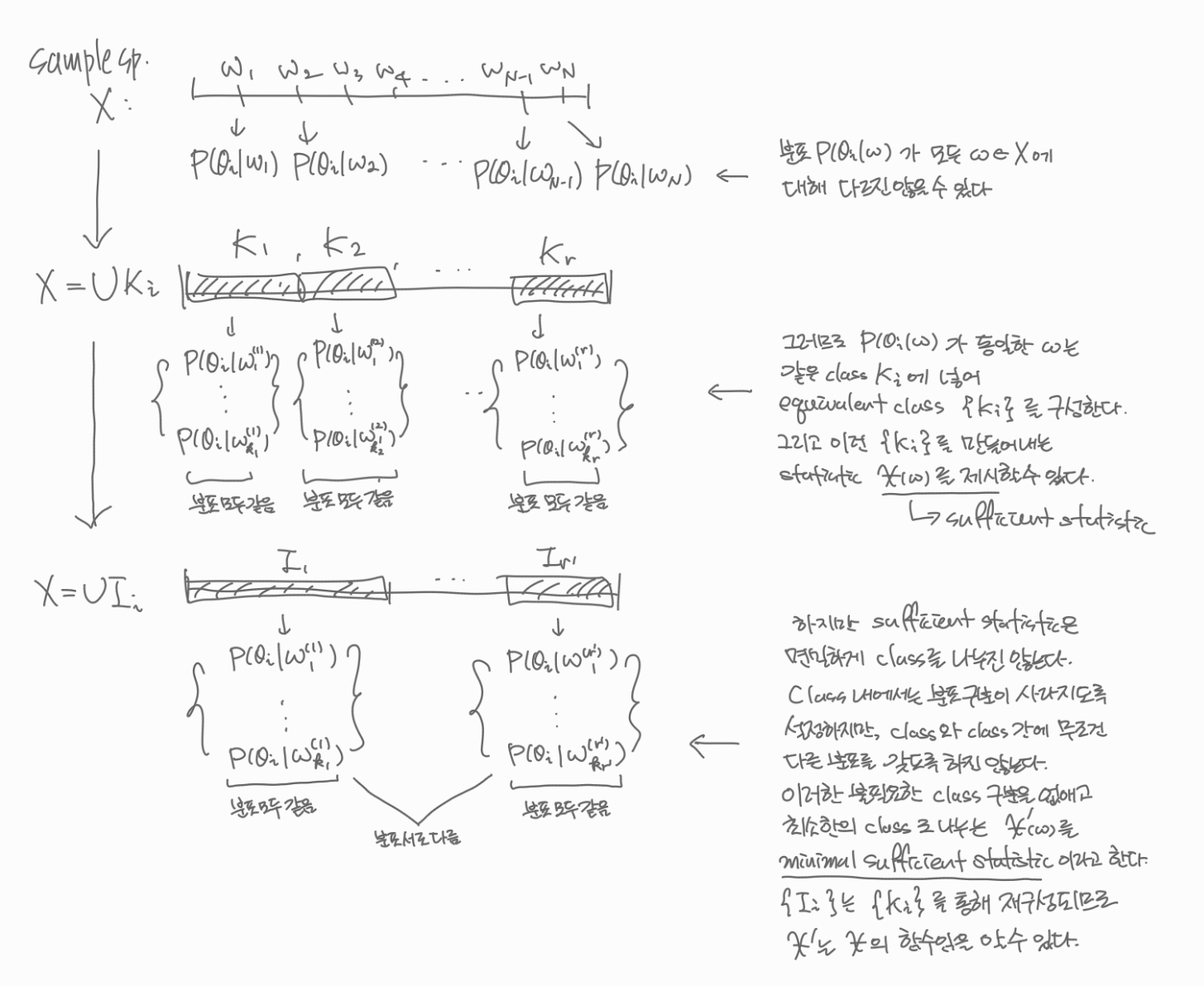
Sufficient statistics의 직관적인 기능의 이해를 돕기 위해서 해당 논문에서는 discrete한 case에 대해서 예시를 제시하였다(이 분야에 특화되지 않은 사람도 이해할 수 있도록 썼다고 본인이 직접 언급했다). 기본적으로 유한한 sample space $X = \left\{w_1, \cdots, w_N\right\}$, 유한한 parameter space $\Omega = \{\theta_1, \cdots, \theta_s\}$에 대하여 family of distribution $\{P_{\theta}(x): \theta\in\Omega\}$를 고려하자. Sample space가 따르는 참(true) 분포가 있고, 이는 어떤 true parameter $\theta_0$에 의해 결정된다고 하자. 즉, 어떤 true parameter $\theta$ 값에 대하여 $P(w_i) = P_{\theta}(w_i)\, (i=1, \cdots, N)$이다.

데이터가 전달하는 정보의 기능을 살펴보기 위해서는 베이즈의 분석 방법만한 것이 없는 것 같다. 그래서 논문 저자도 베이즈의 분석 과정을 차용하여 직관적인 설명을 도모하려고 했던 것이 아닐까 싶다. 각 $\theta\in\Omega$에 대하여 prior distribution이 $P(\theta=\theta_i)=p_i\, (i=1, \cdots, s)$로 가정하였다고 한다면, 랜덤으로 측정된 데이터 $w$에 대하여 우리는 다음의 posterior distribution을 얻는다.

\[P(\theta=\theta_i\vert w) = \frac{p_i P_{\theta_i}(w)}{\sum_{k=1}^sp_kP_{\theta_k}(w)},\quad\quad w\in X,\, i=1, \cdots, s\]

만약 관측된 두 정보 $w’$와 $w^*$에 대하여

\[P_{\theta_i}(w')=P_{\theta_i}(w^*),\quad\quad i=1, \cdots, s\]

였다면, posterior distribution에서의 $w’$와 $w^*$의 값 또한 같을 것이다. 이때 $w’$와 $w^*$를 같은 class에 넣었을 때, 이 과정을 통해 sample space $X$를 equivalent class $K_1, K_2, \cdots, K_r$로 나눌 수 있다. 같은 class에 있는 관측치에 대해서는 임의의 prior distribution(즉, 사전에 어떤 정보가 들어오든 간에)에 대하여 동일한 posterior distribution로 귀결된다면 같은 class에 속한다.

이것이 의미하는 바는 우리가 모든 관측치 $w$를 일일히 따져가면서 통계학적 분석을 할 필요가 없다는 것이다. Posterior distribution이 어느 class에 귀속되는지 알기만 하면 같은 class 내에서는 posterior distribution이 구분되지 않는다(즉, class 안에서는 $\theta_i$에 따른 분포의 구분이 되지 않는다). 그러므로 관측치 $w$의 함수 $\chi(w)$를 적절히 찾아 그 값이 같은 것은 같은 class로 묶고 값이 다른 것은 다른 class로 구분하여 궁극적으로 equivalent class $\{K_i\}$를 찾아내는 것이 관건이다. 이렇게 찾아낸 함수 $\chi$를 sufficient statistic이라고 볼 수 있다.

Sufficient statistic을 정의한 과정을 살펴보면 class 내부에서 분포 사이의 구분이 없도록 구성하지만, class와 class 사이의 분포가 구분되는지에 대해서는 크게 신경쓰지 못했다. 사실은 서로 다른 두 class $K_i$와 $K_j$가 서로 같은 분포를 가지고 있을 수도, 그러므로 불필요한 class 구분이 있을 수 있다. 이를 해결하기 위해서는 우리는 posterior distribution에서 다음을 시도해볼 수도 있다. $\theta_1\in\Omega$에 대하여 $P_{\theta_1}(w)\ne0$이라면,

\[P(\theta=\theta_i\vert w)=\frac{p_i \frac{P_{\theta_i}(w)}{P_{\theta_1}(w)}}{\sum_{k=1}^s p_k\frac{P_{\theta_k}(w)}{P_{\theta_1}(w)}}\]

이때, 두 사건 $w’, w^*\in X$에 대하여

\[\frac{P_{\theta_i}(w')}{P_{\theta_1}(w')}=\frac{P_{\theta_i}(w^*)}{P_{\theta_1}(w^*)}, \quad\quad i=1, \cdots, s\]

면 posterior distribution이 동일해짐을 알 수 있다. 이렇게 equivalent class $\{K_i’\}$를 재구성하게 되면 위에서 구성했던 $\{K_i\}$보다 덜 쪼개지며, 불필요한 class의 구분을 없앨 수 있다. 이런 식의 과정을 통해 class의 구분을 최소화하여 class간의 분포도 다를 수 있도록 equivalent class $\{I_i\}$를 구성하는 statistic $\chi’(w)$를 찾을 수 있을 텐데, 이를 minimal sufficient하다고, 논문의 표현을 빌리면 necessary and sufficient하다고 한다.

그런데 놀랍게도 방금 위에서 제시한 방식은 necessary and sufficient하게 class를 쪼갤 수 있는 방식인데, 이는 일반화하는 과정에서 더 알아보도록 하겠다.

Minimal이라는 표현은 “class의 구분을 최소화하여 정보를 가장 함축적으로 잘 전달하는 statistic”이라는 관점에서 활용되었다고 볼 수 있는데, 기본적으로 정보를 함축해야(즉, 구분되지 않는 분포는 같은 class로 묶어야) 한다는 점에서 sufficient와 함께 쓰여야 할 듯하다. 반면, necessary라는 표현은 “class 별로 분포가 구분될 수 있도록 구성하는 statistic”이라는 관점에서 단독으로 쓰일 수 있지만, necessary statistics는 class 내에에 같은 분포를 가두지는 못한다는 점에서 통계학적으로 활용도가 떨어질 수 있다. 이러한 연유로 necessary라는 표현은 그 기능에 대해선 충분히 잘 붙여진 이름이지만, 결국은 도태되어버리고 minimal sufficient라는 표현이 자리잡게 되었던 것 같다.

위에서 class $\{K_i’\}$를 구성하기 위해서 필요한 statistic $\chi(w)$을 구성하는 방법은 어렵지 않다. 각 $w$에 대하여 class 내에서 대표하는 값들을 mapping해주면 되기 때문이다. 즉,

\[\chi: w\mapsto \left\{\frac{P_{\theta_2}(w)}{P_{\theta_1}(w)}, \frac{P_{\theta_3}(w)}{P_{\theta_1}(w)}, \cdots, \frac{P_{\theta_s}(w)}{P_{\theta_1}(w)}\right\}\]

를 통해 함수값이 같은 $w$들은 같은 class에 속하는 방식이다. 이 mapping 또한 sufficient statistic이라는 성질을 활용하면 discrete한 case에 대해서는 factorization criterion이 쉽게 유도된다.

\[P_{\theta}(w) = P\{\chi(w), \theta\}\cdot Q(w)\]

이렇게 정의한 sufficient statistic이 우리가 알고 있던 정의와 부합하는지도 한 번 살펴보자. Sufficient statistic으로 conditioning을 하면 해당 확률은 parameter와 무관하게 된다. 어떤 class $K_i$가 $\chi(w)=\chi_0$를 만족하는 $w$의 집합이라고 할 때, 우리는 다음을 얻는다.

\[P(w\vert \chi = \chi_0) = \begin{cases} \frac{P_{\theta_i}(w)}{\sum_{w\in K}P_{\theta_i}(w)}, & w\in K; \\ 0, & w\not\in K. \end{cases}\]

Factorization criterion을 활용하면 다음과 같이 된다.

\[P(w\vert \chi = \chi_0) = \begin{cases} \frac{Q(w)}{\sum_{w\in K}Q(w)}, & w\in K; \\ 0, & w\not\in K. \end{cases}\]

그러므로 실제로 parameter와 무관함을 알 수 있고, sufficient statistic의 기능을 충분히 설명한다.

Generalizing the Definition of Sufficiency

Sufficient statistic의 주 기능을 알았기 때문에 일반적인 경우에 대해서도 이 개념을 잘 정립할 수 있게 되었다. 일반적인 정의를 위해서 논문에서 취하는 가정은 다음과 같다(notation은 조금 바꿨다. 논문에서 좀 특이하게 쓴 부분이 있어서..).

$X = \mathbb{R}^m$, parameter space $\Omega$
probability distribution $P_{\theta}(A);\,A\subset X, \theta\in\Omega$
family of probability distribution $\mathcal{P}={P_{\theta}: \theta\in \Omega}$
Definition 1. $\mathcal{P}$ is said to be regular in $B$ if each distribution $P_{\theta}\in \mathcal{P}$ is defined in $B$ by the density $p(x, \theta)$ which is continuous positive function -> $B$ 내에서 density가 존재하고 ‘양수’여야 하며, $B$가 $\theta$에 무관하므로 regular 조건은 다시 말하여 $\mathcal{P}$가 fixed support를 가짐을 의미한다.
Definition 2. $\mathcal{P}$ shall be called piecewise smooth in $B$ if for any $\theta\in\Omega$ the density $p(x, \theta)$ is a piecewise smooth in $B$. -> 주어진 함수 $p(x)$가 piecewise smooth in $I$라고 함은 어떤 domain $O\subset B$가 존재하여 closure $\bar{O}=\bar{B}$이고 $O$에서 $\partial p(x)/\partial x_j$가 존재하고 연속하다는 의미로 정의하였다. -> 이는 곧 $\partial O$를 제외한 나머지에서 first case(일계편도함수)가 존재하고 연속이라는 것이다. $O$의 형태를 예컨대 뚝뚝 끊기는 interval의 합집합이라고 생각하면 piecewise라는 표현이 어울린다. -> 같은 맥락에서 $\partial O$가 굉장히 작은 집합이라고도 볼 수 있지만, 사실 항상 measure-zero set일 필욘는 없다. 이를 테면 $B=[0, 1]$이고 $O$가 cantor set인 경우 Lebesgue $\mu$에 대하여 $\mu(\partial O)\ne 0$이지만 $\partial O$는 uncountable하다. 이러한 문제는 추후 증명에서 사소한 오류로 이어짐을 Brown(1964), Tan(-)이 밝힌 바 있다(이후 리뷰 예정).
$\mathcal{P}$는 별다른 언급이 없으면 regular하고 piecewise smooth하다.

저자는 discrete일 때의 factorization criterion 성질을 확장하여 다음을 일반적인 sufficient statistic의 정의로 삼았다. 요즘은 conditional expectation $E_{\theta}[X\vert \chi(X)]$가 parameter와 무관하게 되는 statistic $\chi(X)$를 sufficient하다고 정의하는 추세이지만, 이 정의와 factorization criterion은 measure thoeretic관점에서도 동치임이 증명되어 있다. 그러므로 사실상 어떤 정의를 차용해도 상관이 없다(저자는 자신의 색다른 접근 방식의 확장을 개연성있게 하기 위해 이렇게 정의한 듯 보인다. 혹은 그 당시 분위기는 이 factorization criterion으로부터 논개하는 분위기가 있었을 수도 있다).

Definition 3. The function $\chi(x)$, defined in the domain $B$ and with values in some set $T$, is called a sufficient statistic in the domain $B$ for the family of distributions $\mathcal{P}$, if the probability densities $p(x, \theta)$ may be put in the form
\[p(x, \theta) = \tilde{p}(\chi(x), \theta)q(x); \quad x\in B,\, \theta\in\Omega.\]

두 statistic $\chi_1(x)$와 $\chi_2(x)$에 대하여 $\chi_1$ being dependent on $\chi_2$하다는 것은 $\chi_2(x’)=\chi_2(x’’)$이면 $\chi_1(x’)=\chi_1(x’’)$가 성립한다는 것이다. 이 표현 역시 저자가 특별히 사용한 표현같은데, 더 간단하게 말하면 $\chi_1$는 $\chi_2$의 함수라는 것이다. 그럼에도 굳이 dependent라는 표현까지 동원한 이유는 불필요한 구분의 class를 합쳐가는 과정이 결국 $\chi_2$에서 $\chi_1$으로 표현되는 것이고, 이를 통해 necessary statistic을 자연스럽게 정의하는 데에 목적이 있다고 생각했다.

Defintion 4. The function $\chi(x)$ is called a necessary statistic for the family of distributions $\mathcal{P}$ in the domain $B$, if it is dependent on every sufficient statistic.

그리고 necessary statistic에 dependent한 statistic은 결국 다시 necessary하다는 것도 자연스레 알 수 있다. 어떤 두 statistic이 서로가 서로에게 sufficient하고 necessary하다는 것이 증명되면 이는 결국 equivalent statistic이 된다. 이러한 의미에서 저자가 지금은 minimal이라고 쓰이는 이 개념을 necessary라고 명명했던 것으로 보인다.

가장 기본이 되는 정리로 어떤 family of distribution에 대하여 necessary and sufficient statistic이 가지는 기본 꼴을 제시하였다. 하지만 이는 언제까지나 기본꼴이며, 여기서 우리는 이 함수를 구성하는 기본적인 ‘재료’를 찾는다면 이들을 뽑아 necessary and sufficient statistic라고 명명할 것이다. 결국은 이 재료들과 $g_x(\theta)$를 모아놓은 space는 equivalent할 것이기 때문이다. 추상적인 발상이지만 아래에 있는 Example 1을 곧 살펴보면서 그 아이디어를 엿보게 된다.

Theorem 1.
\[g_x(\theta) = \log p(x, \theta) - \log p(x, \theta_0); \quad \theta\in\Omega,\]
라고 할 때, 각 $x\in B$에서 함수 $g_x$를 mapping하는 $\chi: x\mapsto g_x(\theta)$는 necessary and sufficient statistic이다.

증명은 간단하게 할 수 있다.

$g_x$ is sufficient: $p(x, \theta) = e^{g_x(\theta)}p(x, \theta_0)$ and was to be proved by Definition 3.
$g_x$ is necessary: for each sufficient $\chi(x)$ and by Definition 3 that $p(x, \theta)=\tilde{p}(\chi(x), \theta)q(x)$, $g_x(\theta) =\log \left[\tilde{p}(\chi(x), \theta) / \tilde{p}(\chi(x), \theta_0)\right]$ which is dependent on $\chi(x)$.

예컨대 $\Omega$가 유한집합이라면 $\chi$는 각 $x$에 대하여 vector를 mapping하는 것으로 재표현할 수 있다. 즉,

\[\chi: x\mapsto (g_x(\theta_1), \cdots, g_x(\theta_r))\]

인 셈이다. 이러한 면에서 앞에서 equivalent class 내의 대표값과 mapping으로 도출한 논의와 일맥상통함을 알 수 있다.

참고로 만약 데이터가 $n$개의 iid한 observation $(x_1, \cdots, x_n)$으로 이루어져 있다면, necessary and sufficient statistic은 다음과 같이 직관적으로 표현될 수 있다.

\[g_{x_1, \cdots, x_n}(\theta) = g_{x_1}(\theta)+\cdots +g_{x_n}(\theta)\]

Example 1. 정규분포 $N(\mu, \sigma^2)$로부터 iid하게 추출된 sample $X_1, \cdots, X_n$에 대해 살펴보자. 고정된 $\theta_0=(\mu_0, \sigma_0^2)$에 대하여 theorem 1에서 제시한 necessary and sufficient statistic를 구하면

\[g_{x_1, \cdots, x_n}(\mu, \sigma^2) = -\frac{1}{2}\left(\frac{1}{\sigma^2}-\frac{1}{\sigma_0^2}\right)\sum x_i^2 + \left(\frac{\mu}{\sigma^2}-\frac{\mu_0}{\sigma_0^2}\right)\sum x_i - \left(\frac{\mu^2}{2\sigma^2}-\frac{\mu_0}{2\sigma_0^2}+\log\frac{\sigma}{\sigma_0}\right)\]

즉, $(x_1, \cdots x_n)\mapsto g_{x_1, \cdots, x_n}(\mu, \sigma^2)$는 $(\sum x_i^2, \sum x_i, 1)$의 선형결합으로 표현될 수 있다. 곧, function space $\{g_{x_1, \cdots, x_n}(\mu, \sigma^2): (\mu, \sigma^2)\in\mathbb{R}\times\mathbb{R}^+\}$ (여기서 유의할 점은 이 space의 함수는 $(x_1, \cdots x_n)\mapsto g_{x_1, \cdots, x_n}(\mu, \sigma^2)$이고, $(\mu, \sigma^2)$은 함수의 label이다… 이렇게 따지면 사실 $g_{\mu, \sigma^2}(x_1, \cdots, x_n)$이 더 맞는 표현이겠지만 $g$는 이후 세대에서 log-likelihood라는 이름이 붙으며 parameter의 함수로 쓰이기 때문에 그 관습에 맞춘 것뿐이다)는 $\{\phi_1(x), \phi_2(x), 1\}=\{\sum x_i^2, \sum x_i, 1\}$를 basis로 갖는다. 즉, 이들은 $g_{x_1, \cdots x_n}(\theta)$를 선형결합으로 구성한다는 관점에서 기본적인 ‘재료’이다. 그러므로 $\chi$를 $\{\phi_1, \phi_2\}$로 재표현해도 equivalent하다는 것을 직관적으로 알 수 있다.

물론 엄밀한 증명이 필요하고 이는 곧 다루게 된다! 여기서 강조하고 싶은 것은 function space의 적절한 basis를 찾는 과정을 통해 그 구조를 파악할 수 있다는 것이다. 또한 데이터는 $n$개인데 basis는 3차원인 것을 보면 분명 차원 축소가 있었다는 것인데 차원 축소는 항상 가능한 것인지, 가능하다면 어떤 형태로 나타나는지에 대해 궁금증을 유발한다.

Advent of the Exponential Family

위에 있는 example 1에서 보았듯이 우리는 ${g_x(\theta): \theta\in \Omega}$로 주어지는 function space에 대한 분석이 필요하다. 이 space의 dimension이 유한하다면 우리는 적절한 basis function을 찾을 수 있을 터인데, 이는 곧 $\chi$와 equivalent한 necessary and sufficient statistic이 됨을 직관적으로 알 수 있었다. 아래에서 소개할 theorem 2은 이를 정형화한 것이다.

소개하기에 앞서 잠시 dimension에 대해 조금 더 살펴보자. Function space ${g_x(\theta): \theta\in \Omega}$의 dimension을 $r+1$이라고 하고(즉, 상수함수를 제외하고도 $r$개의 basis 함수를 찾을 수 있다), 우리는 $n$개의 sample을 iid로 추출하였다고 하자. 다음 두 경우를 살펴볼 수 있다.

$n \ge r$. 굳이 $n$개의 데이터를 직접 활용할 필요 없이 $r$차원의 necessary and sufficient statistic을 활용함으로써 dimension reduction을 할 수 있다.
$n<r$. Data reduction을 해봐야 데이터 차원보단 높을 수밖에 없는 상황이다. 모름지기 $n$개의 데이터를 직접 활용하여도 그 자체로 sufficient statistic일 것이며, 그럼에도 데이터 차원이 부족하기 때문에 class를 necessary 조건을 만족하도록 나누지 못할 수 있다.

이를 바탕으로 theorem 2가 정립되었고, 이는 이 논문에서뿐만 아니라 앞으로 family of distribution의 rank를 논의하는 데에 중추 역할을 한다.

Theorem 2 (The Form of Necessary and Sufficient Statistics). Let the system $\mathcal{P}$ of one-dimensional probability distributions be regular and piecewise smooth in the interval $I$. We shall denote by $L(\mathcal{P}, I)$ the minimal linear space of functions, defined in $I$, consisting of constants and functions $g_x$. Let the dimension of $L(\mathcal{P}, I)$ be $r+1$(including the case $r=\infty$). Then
For every finite $n\le r$ any sufficient statistic for a smple of size $n$ is trivial.
If the functions $1, \phi_1(x), \cdots, \phi_r(x)$ are bases in $L(\mathcal{P}, I)$ then for any $n\ge r$ the system of functions
\[\chi_i(x_1, \cdots x_n) = \phi_i(x_1)+\cdots +\phi_i(x_n); \quad i=1, \cdots, r,\]
is functionally independent and forms a necessary and sufficient statistic for the sample of size $n$.

이때 sufficient statistic이 trivial하다는 것은 데이터와 one-to-one mapping이 있음을, 즉 그 데이터 자체를 dimension의 reduction 없이 sufficient statistic으로 활용한다는 것이다. 예컨대 order statistics $\chi_i(x_1, \cdots, x_n) = x_{(i)}$는 trivial statistic이다.

증명은 간략히 다음 흐름을 따른다.

$\chi(x_1, \cdots, x_n)$ is dependent on $g_{x_1, \cdots, x_n}(\theta)$ : $\phi(x)\in L$이면 $\phi$는 $\{g(\theta_q)\}_q$들의 선형결합이므로 $\chi$도 그 선형결합으로 표현 가능하다.
$g_{x_1, \cdots, x_n}(\theta)$ is dependent on $\chi(x_1, \cdots, x_n)$: $\{1, \phi_1, \cdots, \phi_s\}$가 $L$를 generate할 때(꼭 basis를 지칭하는 것이 아니다), 각 $\theta\in\Omega$에 대하여 $g_x(\theta)\in L$은 $1$과 $\phi_i(x)$의 선형결합으로 표현 가능하다. 따라서 $g_{x_1, \cdots, x_n}(\theta)$도 $\{\sum_j \phi_i(x_j)\}_i$의 선형결합, 즉 $\{\chi_i\}_i$의 선형결합으로 표현할 수 있다.
$n\ge s$에 대하여 $\{1, \phi_1, \cdots, \phi_s\}$가 $L$에서 linearly independent하다면 $\chi_i(x_1, \cdots, x_n) = \sum_j \phi_i(x_j)\, (i=1, \cdots, s)$ 또한 linearly independent하다:
- 귀류로 접근하여 $\chi_i$가 linearly dependent하다고 하자.
- 함수 $F$가 있어 $F(\chi_1, \cdots, \chi_s)=0$가 성립하고 Jacobian $\partial F(\chi_1, \cdots, \chi_s)/\partial(x_1, \cdots, x_s) = \vert \{\phi’i(x_j)\}{ij} \vert =0$이다. 이 경우 $\{1, \chi_1, \cdots, \phi_s\}$가 linearly dependent함을 귀납적으로 증명 가능.
  - $\partial(\chi_1, \cdots, \chi_{s-1})/\partial (x_1, \cdots, x_{s-1})=0$인 경우는 귀납가정에 의해 성립.
  - 그 외의 경우를 갖는 점 $x^0=(x_1^0, \cdots, x_{s-1}^0)$에 대해, determinant를 마지막 열을 기준으로 전개하면 $\partial F(\chi_1, \cdots, \chi_s)/\partial(x_1, \cdots, x_s)=A_1\phi_1’(x) + \cdots + A_s\phi_s’(x)=0$이 성립. 이때 $A_i$는 고정 상수 $x^0$와만 관련있고, $x$의 함수는 아님. 또, $A_s\ne 0$.
  - Piecewise 조건에 의해 $A_1\phi_1(x) +\cdots + A_s\phi_s(x)$는 구간마다 상수의 값을 가짐. 곧 continuity 조건에 의해 이 상수값들은 전부 같아야함(하지만 이 논리는 사소한 오류가 있음이 Brown(1964), Tan(-)에 의해 밝혀짐. 끊기는 구간에서 다른 상수값을 가져도 continuity는 유지될 수 있기 때문. Cantor function을 예로 살펴볼 수 있다. 이는 곧 piecewise 조건만으로는 부족하다는 것을 의미한다! 이 때문에 앞으로의 정리에서 계속 나오는 piecewise smooth 조건은 모두 불충분하며, 하나의 interval에서 continuously differentiable로 가정하거나 $\partial O$가 countable하다고 가정해야 한다).
- 조건에 모순이므로 원명제가 성립.
(a)의 경우, $n<r$이므로 linearly independent한 $\{1, \phi_1, \cdots, \phi_n\}$를 적절히 고를 수 있다. 3번에 의해($s=n$인 경우) $\{\chi_1, \cdots, \chi_n\}$도 linearly indepedent하다. 따라서 어떤 점 $x^0=(x_1^0, \cdots, x_n^0)$에 대해 Jacobian $\partial F(\chi_1, \cdots, \chi_n)/\partial(x_1, \cdots, x_n)\ne 0$이므로 $F$가 invertible하여 $x_i = x_i(\chi_1, \cdots, \chi_n)$ 인 $x_i$가 존재, 즉 해당 sufficient statistic은 trivial 하다.
(b)의 경우, 1번과 2번에 의해 $\{\chi_i\}_{1\le i\le r}$는 necessary and sufficient하며, 3번에 의해($s=r$인 경우) linearly independent하다.

이를 바탕으로 저자는 family of distribution의 rank를 정의했다.

Definition 5. The rank of a system of distributions $\mathcal{P}$ in the domain $B$ is defined as the greatest $r$, such that for any finite $n\le r$ the family $\mathcal{P}$ has no non-trivial sufficient statistics for the sample of size $n$ in the domain $B$.

즉, 데이터의 전부를 sufficient statistics로 활용해야만 family of distribution을 설명할 수 있는 최대의 데이터 개수를 rank로 본 것이다. 이는 sufficient statistics의 차원이 곧 family of distribution의 정보의 차원이라는 고유한 특성임을 인식시켜 준다.

이러한 관점에서 finite rank를 갖는 family of distribution은 결국 exponential family에 속할 수밖에 없음을 다음 정리에서 보여준다. 이는 다시 말하여 data reduction이 가능하다면 exponential family꼴일 수밖에 없음을 의미(물론 충분한 regularity 아래에서 말이다)한다. Exponential family가 sufficient statistic에서 주목받을 수밖에 없는 진정한 이유를 여기에서 바라볼 수 있게 된다.

Theorem 3 (Finite Rank => Exponential Family). If the system of distributions $\mathcal{P}$ is piecewise smooth and has finite rank $r$ in the interval $I$, then the density $p(x, \theta)$ can be written in the form
\[p(x, \theta) = \exp\left[\sum_{i=1}^r\phi_i(x)c_i(\theta)+c_0(\theta)+\phi_0(x)\right]; \quad x\in I, \theta\in\Omega,\]
where the functions $\phi_1(x), \cdots, \phi_r(x)$ are picewise smooth in the interval $I$ and the system of functions $(1, \phi_1, \cdots, \phi_r)$ and $(1, c_1, \cdots, c_r)$ are linearly independent.

증명은 다음 흐름을 따른다.

$L$의 basis $\{1, \phi_1, \cdots, \phi_r\}$가 있다고 하면, 각 $\theta\in\Omega$에 대해 $g_x(\theta)$는 이들의 선형결합으로 표현된다.
- $g_x(\theta) = \sum_{i=1}^r c_i(\theta)\phi_i(x) + c_0(\theta) =\log[p(x, \theta)/p(x, \theta_0)]$
- 정리하면 우리가 원하는 $p(x, \theta)$를 얻음.
$\{1, \phi_1, \cdots, \phi_r\}$은 이미 independent. $\{1, c_1, \cdots, c_r\}$이 independent한 것만 증명하면 된다.
- 만약 independent하지 않는다면, 직관적으로 $L$이 $r+1$개보다 적은 basis로도 표현 가능함을 알 수 있음. 하지만 이를 한편으론 당연하지 않을 수 있는 과정인 reference point로 처리하는 세밀한 과정을 살펴보도록 하자.
- $c_r(\theta)=b_0+b_1c_1(\theta)+\cdots b_{r-1}c_{r-1}(\theta)$의 관계를 찾을 수 있음.
- $g_x(\theta)=\sum_{i=1}^{r-1}c_i(\theta)\phi_i^*(x)+c_0(\theta)+b_0\phi_r(x)$으로 재표현 가능.
- 정의상 $g_x(\theta_0)=0$이므로 $g_x(\theta)=g_x(\theta)-g_x(\theta_0)=\sum_{i=1}^{r-1}[c_i(\theta)-c_i(\theta_0)]\phi_i^*(x)+c_0(\theta)-c_0(\theta_0)$ (reference point $\theta_0$를 활용하여 $b_0\phi_r(x)$ 항을 처리함. $\theta$로 labeling된 함수들로써 basis의 계수가 $\theta$에 대한 함수가 아니라면 결국 $\phi_r(x)$는 상수항임.)
- rank $L < r+1$, 모순.

이제 그 역이 성립함을 살펴볼 것이다. 즉, exponential family는 rank가 유한하며, 때문에 trivial하지 않은 necessary and sufficient statistics를 가진다. Exponential family는 그러므로 dimension reduction이 가능한 유일한 family임을 알 수 있다.

Theorem 3a (Exponential Family => Finite Rank). Let
\[p(x, \theta) = \exp\left[\sum_{i=1}^r c_i(\theta)\phi_i(x)+c_0(\theta)+\phi_0(x)\right];\quad x\in I, \theta\in\Omega,\]
where $\phi(x)$ are piecewise smooth functions.
The the rank of the system $\mathcal{P}$ does not exceed $r$.
If $(1, \phi_1, \cdots, \phi_r)$ and $(1, c_1, \cdots, c_r)$ are linearly independent system of functions, then the rank of $\mathcal{P}$ equals $r$, and
for any $n\ge r$ the system of functions $\chi_i(x_1, \cdots, x_n) = \sum_{j=1}^n \phi_i(x_j);\quad i=1, \cdots, r,$is functionally independent and forms a necessary and sufficient statistic for the family $\mathcal{P}$ for the sample of size $n$.

증명은 간략히 다음과 같다.

주어진 density 꼴로부터 $g_x(\theta)=\sum_{i=1}^r(c_i(\theta)-c_i)\phi_i(x)+(c_0(\theta)-c_0)$, $c_i=c_i(\theta_0)$.
- $L(\mathcal{P}, I)$의 차원은 $\le r+1$이므로 $\mathcal{P}$의 rank도 $\le r$.
$(1, \phi_1, \cdots, \phi_r)$ and $(1, c_1, \cdots, c_r)$ are linearly independent하면 $\{1, \phi_1, \cdots, \phi_r\}$이 $L$의 basis가 됨을 보이자.
- $(c_1(\theta)-c_1, \cdots, c_r(\theta)-c_r)$은 linearly independent -> $\theta_1, \cdots, \theta_s\in\Omega$를 적절히 찾아서 determinant $\vert \{c_i(\theta_j)-c_i\}_{ij}\vert\ne0$이도록 만들 수 있음.
- 연립방정식 $\{g_x(\theta_j)\}_j=\{c_i(\theta_j)-c_i\}_{ij}\{\phi_i(x)\}_i+\{c_0(\theta_j)-c_0\}_j$은 solvable함.
- $\phi_i(x)$는 $g_x(\theta_j)$의 선형결합으로 표현되므로 $\phi_i\in L$.
- Independence 조건, $g_x(\theta)$가 항상 $\phi_i$의 선형결합으로 표현됨, $\phi_i\in L$로부터 $\{1, \phi_1, \cdots, \phi_r\}$은 $L$의 basis.
이후 $n\ge r$인 경우 Theorem 2를 따름.

논문에서는 친절하게 이에 대한 예시도 함께 제시하였다.

Example 2a. Parameter $0<\mu<+\infty$와 고정된 상수 $\beta, \lambda$에 대하여 다음 꼴의 density

\[p(x, \mu) = \begin{cases} Cx^{\beta}e^{-\lambda x^{\mu}}, & x>0; \\ 0, & x\le 0, \end{cases}\]

를 가지는 distribution의 family $\mathcal{P}$를 고려하자. 이는 $I=(0, +\infty)$에서 regular(즉, fixed support)하며, $\mathbb{R}\setminus O$에서 smooth하다. Log-likelihood 꼴의 necessary and sufficient statistic은

\[g_x(\mu) = -\lambda x^{\mu}+(\log C -\log C_0 + \lambda x^{\mu_0}),\]

이다. 따라서 function space $L(\mathcal{P}, I)$는 $\phi_\mu(x) = x^{\mu}$에 대한 linear system임을 알 수 있다. 하지만 각각의 $\mu$에 대해서 $\phi_\mu$는 서로 functionally independent하기 때문에 결국 $L$은 무한 차원을 갖는다. 그러므로 family $\mathcal{P}$ 또한 infinite rank를 가지고 있다. $\mu$의 parameter space를 어떤 유한한 범위 $(\mu_1, \mu_2)$로 제한시켜도, 혹은 지금은 상수로 주어진 $\beta$나 $\lambda$를 parameter로 취급할 때에도 $\mathcal{P}$이 infinite rank를 갖는다는 사실엔 변함이 없다. 이것이 한편 의미하는 것은 density가 위와 같은 꼴이라면 trivial한 형태를 제외하고는 다른 형태의sufficient statistic를 절대 도출할 수 없으며, 따라서 정보의 함축이 불가능하고 데이터 $n$개의 데이터를 곧이곧대로 활용하는 것이 최선이라는 것이다.

만약 $\mu$가 parameter가 아닌 주어진 상수로 취급되면 어떨까? $\beta$와 $\lambda$가 상수냐 parameter에 따라 우리는 다음의 necessary and sufficient statistic을 얻을 수 있다. 즉, 이 경우에는 dimension reduction이 가능하다.

unknown $\beta$, known $\lambda$: $\sum_{i=1}^n \log x_i$
known $\beta$, unknown $\lambda$: $\sum_{i=1}^n x^{\mu_i}$
unknown $\beta$, $\lambda$: $\left(\sum_{i=1}^n \log x_i, \sum_{i=1}^n x^{\mu_i}\right)$

Example 2b. Laplacian family of distribution $\mathcal{P}$의 density 꼴은

\[p(x, \alpha, \sigma)=\frac{1}{2\sigma} \exp\left[\frac{\vert x-\alpha\vert}{\sigma}\right],\]

으로 정의된다. 이때 log-likelihood 꼴의 necessary and sufficient statistic의 형태는 다음과 같다.

\[g_x(\alpha, \sigma) = -\log\frac{\sigma}{\sigma_0} -\frac{\vert x-\alpha\vert}{\sigma}+\frac{\vert x-\alpha_0\vert}{\sigma_0}\]

$\alpha$가 고정된 상수라면 이 family의 necessary and sufficient statistic은 $\sum_{i=1}^n \vert x_i-\alpha\vert$이다.
$\alpha$가 알려지지 않은 parameter라면 $L(\mathcal{P}, I)$는 independent한 함수 $\vert x-\alpha\vert$로부터 span된다. 즉, 임의의 interval $I$에 대하여 $L(\mathcal{P}, I)$은 infinite rank를 갖는다.

Exponential Location Family

지금까지 exponential family의 꼴과 그 특징에 대해 살펴보았다. 느꼈을지 모르겠지만, 주어진 dimension을 갖는 function space $L(\mathcal{P}, I)$를 분석하는 과정은 결국 통계학보다는 함수해석학에 가까운 과정이다. 어떤 function space가 갖춰져야 하는 함수꼴이 있을 때, 그럼에도 finite dimension을 갖기 위해서 필연적으로 가져야만 하는 basis의 꼴에 대해 앞으로 살펴볼 것이다.

이를테면 location family가 finite dimenson을 가진다고 하자. 아무튼 $L$이 finite dimenson이기 때문에 필연적으로 해당 family는 exponential일 수밖에 없다. 즉, 우리는 exponential family이면서 location family임을 찾는 것이나 다름없다.

Location family는 결국 $\mathcal{P}$에 속한 distribution의 density $f$가 모두 어떤 하나의 함수 $F$에 대하여 $f(x, \alpha)=F(x-\alpha)$ 꼴로 표현됨을 의미한다. 예컨대 위에서 살펴본 Example 2b에서 $x$에 대한 함수의 family $\{\vert x - \alpha\vert, \alpha\in\mathbb{R}\}$을 고려할 수 있다. 이 family는 각각의 $\alpha$에 대해서 $\vert x-\alpha\vert$가 모두 서로 independent하기 때문에 dimension이 무한하다. 짐작컨대 $\alpha$에 따른 $f(x-\alpha)$들을 모아놓은 space가 유한한 차원이기 위해서는, 즉 유한 개의 basis들의 선형결합으로 표현되기 위해서는 $f$가 $x-\alpha$의 함수여야 한다는 제약 탓에 굉장히 특별한 꼴이어야 할 것이다.

Lemma 1. Let $a<a’<b’<b$, $\delta<\min(a’-a, b’-b)$. Let the function $f(x)$ be defined and picewise smooth in the interval $I=(a, b)$. If the family of functons $f(x-\alpha)$, where $x\in I’=(a’, b’)$, $\vert\alpha\vert <\delta$ has a linear system of finite dimension, then
\[f(x) = \sum_{i=1}^s c_i x^{n_i}e^{\mu_i x}; \quad x\in I',\]
where $c_i, \mu_i$ are complex constants and $n_i$ are integral constants.

원문에는 $f$의 꼴이 $\sum_{i=1}^s[c_i-x^{n_i}e^{\mu_i x}]$로 주어진다고 했는데, 아무리 봐도 오타인 듯하다. 증명은 간략히 다음 흐름을 따른다.

$f_i(x) = f(x-\alpha_i)\in L\, (i=1, \cdots, k)$이 $L$를 span하는 independent한 함수라고 하자.
얼추 작은 $\lambda$에 대하여 $\vert t\vert <\lambda$, $x\in I’$에 대해
- $f_i(x-t) = f(x-\alpha_i-t) = \sum_{j=1}^k a_{ij}(t)f_j(x);\quad i=1, \cdots, k$
Determinant $\vert \{f_j(x_l)\}_{jl}\vert\ne 0$이고 $f_j(x)$가 $x_l$에서 differentiable한 $x_l\in I’\,(l=1, \cdots, k)$를 잡자. 위의 식에 $x_l$들을 대입하여 각 $i$에 대해 연립방정식을 만들자.
- $\{f_i(x_l - t)\}_l = \{f_j(x_l)\}_{jl}\{a_{ij}(t)\}_j$
- $\{a_{ij}(t)\}_j = \{f_j(x_l)\}_{jl}^{-1}\{f_i(x_l - t)\}_l$으로 표현 가능 => $\alpha_{ij}$는 $t=0$에서 differentiable.
따라서 첫번째 관계식의 $t=0$에서 미분계수는(이때 $A_{ij}=-\alpha_{ij}’(0)$):
- $f’_i(x) = \sum_{j=1}^k A_{ij}f_j(x); \quad x\in I’, \, i=1, \cdots, k$
간단한 선형 미분방정식임. $f$는 결국 위와 같은 꼴이 나옴.
- $[A_{ij}]$의 eigenvalue $\mu$가 $n+1$의 multiple을 가지고 있다면 $e^\mu, xe^\mu, \cdots, x^ne^\mu$의 선형결합으로 표현됨.

다음 Theorem 4은 Lemma 1을 기반으로 한다.

Theorem 4 (Exponential Location Family). Let there be established a distribution function $F(x, \theta)$ for every $\theta\in\Omega$. Let the family $\mathcal{P}$ of these distributions be regular and piecewise smooth in the interval $I=(a, b)$. If for some positive $\delta$ the family $\mathcal{P}_{\delta}$ of distributions $F(x-\alpha, \theta)$ $(\theta\in\Omega, \vert\alpha\vert <\delta)$ has finite rank in $I$, then the density $p(x, \theta)$ can be put in the form
\[p(x, \theta) = \exp\left[\sum_{i=1}^s c_i(\theta)x^{n_i}e^{\mu_i x}\right]; \quad x\in I,\, \theta\in \Omega.\]

결국 우리가 찾고자 하는 family는 $\mathcal{P}_{\delta}$이다. 이때 $\alpha$를 location parameter라고 하며, 여기서 $\delta$는 고정된 support가 한정된 범위를 갖기 때문에 붙여진 부가적인 요소로써, 이는 처음부터 어떤 값으로 고정되지만 density의 꼴에 결국 영향을 주진 않는다(엄밀성을 위해 있는 장치이므로 크게 신경쓰지 않아도 될 듯).

증명은 다음 흐름을 따른다.

$\mathcal{P}$보다 $\mathcal{P}_\delta$에 더 많은 distribution이 포함되어 있으므로 $\text{rank }\mathcal{P}<\text{rank }\mathcal{P}_\delta<\infty.$
- Theorem 3에 의해 $\mathcal{P}$는 exponential family.
- $\log p(x, \theta) = \sum_{i=1}^r c_i(\theta)\phi_i(x)+c_0(\theta)+\phi_0(x); \quad x\in I, \,\theta\in\Omega.$
위의 식으로부터 $\log p(x-\alpha, \theta) = \sum_{i=1}^r c_i(\theta)\phi_i(x-\alpha)+c_0(\theta)+\phi_0(x-\alpha); \quad \theta\in\Omega,\, \vert\alpha\vert<\delta,\, x\in I’.$
- 이때 $a<a’<b’<b$, $I’=(a’, b’)$.
- 그러므로 $L(\mathcal{P}_{\delta}, I’)$은 다음 함수를 모아놓은 function space임. $\begin{align}g_x(\alpha, \theta) &=\log p(x-\alpha, \theta)-\log p(x-0, \theta_0)\\ &=\sum_{i=1}^r c_i(\theta)\phi_i(x-\alpha)-\sum_{i=1}^rc_i(\theta_0)\phi_i(x) +c_0(\theta)+\phi_0(x-\alpha)-\phi_0(x)-c_0(\theta_0)\end{align}$
- $\text{rank }\mathcal{P}_{\delta}<\infty$, 위의 $g_x(\alpha=0, \theta)$의 꼴로부터 Theorem 3a의 두 번째 항목 증명 흐름과 비슷한 과정으로 $\phi_i(x)\in L(\mathcal{P}_{\delta}, I’)$ 임을 보일 수 있음.
결국 $\sum_{i=1}^r c_i(\theta)\phi_i(x-\alpha)+\phi_0(x-\alpha)-\phi_0(x)\in L(\mathcal{P}_{\delta}, I’)$.
- 다시 Theorem 3a 두 번째 항목과 같은 논리로 $\phi_i(x-\alpha), [\phi_0(x-\alpha)-\phi_0(x)]\in L(\mathcal{P}_{\delta}, I’)$
- 원문엔 바로 위 두 식이 각각 $\in L(\mathcal{P}, I’)$, $\in L(\mathcal{P}_j, I’)$으로 되어 있었는데 아무리 봐도 오타인 듯.
$L(\mathcal{P}_{\delta}, I’)$ 안에 $\phi_i(x-\alpha)$ 꼴이 모두 포함되어 있으므로 Lemma 1에 의해 $\phi_i$ 꼴이 특정됨.
- $\phi_i(x) = \sum_{j=1}^{s_i} c_j^{(i)} x^{n_j^{(i)}}e^{\mu_j^{(i)}x}; \quad i=0, \cdots, r;\, x\in I’.$
- $\phi_i$는 $I’$ 위에서 analytic, $a’\searrow a$, $b’\nearrow b$로 취해도 위 논리 성립, $I$로의 정의역 확장 가능.
따라서 $\log p(x-\alpha, \theta)=\sum_{i=1}^s c_j(x-\alpha)^{n_j}e^{\mu_j(x-\alpha)}$. 보이고자 하는 바가 증명됨.

Exponential family를 유도할 때도 그랬듯이, exponential location family도 그 역이 성립함을 증명할 수 있다. 이로서 해당 family에서 necessary and sufficient statistic의 꼴이 특정된다.

Theorem 4a (Exponential Location Family, the Converse). Let the distribution of the class $\mathcal{P}$ be given in the interval $I=(a, b)$ by densities of the type
\[p(x, \theta) = \exp\left[\sum_{i=1}^t Q_i(x, \theta)e^{\lambda_i x} +Q_0(x, \theta) \right]; \quad \theta\in \Omega,\]
where $\lambda_1, \cdots, \lambda_t$ are non-zero complex numbers, different in pairs and $Q_i(x, \theta),\, i=0, \cdots, r$ polynomials of degree $k$, in $x$. Let $a<a’<b’<b$ and $\delta<\min{a’-a, b’-b}$. Then
the distributions $p(x-\alpha, \theta);\,\theta\in\Omega,\,\vert\alpha\vert<\delta$ form a family of finite rank $r$ in the interval $I’=(a’, b’).$
Let $Q_0(x, \theta)= A(\theta)x^{k_0}+\cdots$, where the row of dots is occupied by terms of degree less than $k_0$. Then,
if $k_0>0$ and $A(\theta)$ is constant for all $\theta\in\Omega$, $r=(k_0-l)+\sum_{i=1}^t (k_i+1)$, and $\chi_{\lambda_i}^{l_i}\, (i=1, \cdots, t;\, 0\le l_i\le k_i);\,\chi_0^{l_0}\,(0<l_0<k_0)$ is the necessary and sufficient statistic, and
if not, $r=k_0+\sum_{i=1}^t (k_i+1)$ an $\chi_{\lambda_i}^{l_i}\,(i=1, \cdots, t;\, 0\le l_i\le k_i);\,\chi_0^{l_0}\, (0<l_0\le k_0),$ is the necessary and sufficient statistic,
where $\chi_{\lambda}^{l}(x_1, \cdots, x_n) = \sum_{j=1}^n x_j^{l}e^{\lambda x_j}$.

이를 증명하기 위해서는 먼저 다음 간단한 Lemma 2가 필요하다.

Lemma 2. Let $\lambda_1, \cdots, \lambda_t$ be complex numbers, different in pairs, and let $Q_1(x), \cdots, Q_t(x)$ be rational funcitons with complex coeffiecients. If in some interval
\[\sum_{i=1}^t Q_i(x) e^{\lambda_i x} =0\]
identically, then the functions $Q_1, \cdots, Q_t$ are identically zero.

증명은 간략히 다음 과정을 따른다.

귀납적으로 $t-1$일 때 성립한다고 가정하자.
준식을 $Q_t(x) e^{\lambda_tx}$으로 나누면($Q_t=0$이면 trivial, assume otherwise) $\sum_{i=1}^{t-1} \tilde{Q}_i(x)e^{\tilde{\lambda}_ix}+1=0$.
- 이때 $\tilde{Q_i}=Q_i/Q_t$도 rational, $\tilde{\lambda}_i=\lambda_i -\lambda_t\ne 0$.
위 식을 미분하면 $\sum_{i=1}^{t-1} (\tilde{Q}_i’+\tilde{\lambda}_i\tilde{Q}_i)e^{\tilde{\lambda}_i x}=0$.
귀납 가정에 의해 $\tilde{Q}_i’+\tilde{\lambda}_i\tilde{Q}_i=0; \quad i=1, \cdots, t-1.$
$\tilde{Q}_i=c_ie^{\tilde{\lambda}_ix}$이고 $\tilde{\lambda}_i\ne0$이라는 점에서 $c_i=0$이어야만 $\tilde{Q_i}$이 rational.
- $Q_1, \cdots, Q_{t-1}\equiv0$ implies $Q_t\equiv 0$.

자, 이제 Lemma 2를 바탕으로 Theorem 4a을 증명하는 과정을 살펴보자.

$\log p(x-\alpha. \theta)=\sum_{i=1}^t Q_i(x-\alpha, \theta)e^{\lambda_i(x-\alpha)}+Q_0(x-\alpha, \theta);\quad x\in I’,\, \theta\in\Omega,\,\vert \alpha\vert<\delta.$
$Q_i(x-\alpha, \theta)$를 $x=0$을 기준으로 Taylor 전개를 한다.
- $Q_i(x-\alpha) = \sum_{l_i=0}^{k_i} c_{l_i}^{(i)}(\alpha, \theta) x^{l_i}$ where $c_{l_i}^{(i)}(\alpha, \theta)=\frac{1}{l_i !}\frac{\partial^{l_i}Q_i}{\partial x^{l_i}}(-\alpha, \theta); \quad i=0, \cdots, t.$
- 식을 정리하면 $\begin{align}\log p(x-\alpha, \theta) &= \sum_{i=1}^t\sum_{l_i=0}^{k_i}c_{l_i}^{(i)}(\alpha, \theta)e^{-\alpha\lambda_i}\cdot x^{l_i}e^{\lambda_i x}\\+&\sum_{l_0=1}^{k_0-1} c_{l_0}^{(0)}(\alpha, \theta)\cdot x^{l_0} +A(\theta)\cdot x^{k_0} + c_0^{(0)}(\alpha, \theta)\end{align}$
Lemma 2에 의하여
- $1,\, x^{l_i}e^{\lambda_i x}(i=1, \cdots, t;\, 0\le l_i\le k_i),\, x^{l_0} (0<l_0\le k_0)$는 서로 independent.
- $1,\,c_{l_i}^{(i)}(\alpha, \theta)e^{-\alpha\lambda_i} (i=1, \cdots, t;\, 0\le l_i\le k_i),\, c_{l_0}^{(0)} (0<l_0<k_0)$도 서로 independent
- $A(\theta)$가 constant가 아니라면 위 두 개의 함수 묶음에서 각각 $x^{k_0}$와 $A(\theta)$도 independent함.
이후 Theorem 2에 따름.

Exponential Group Family

비단 location family 뿐만이 아니라 $F(x/\sigma)$ 꼴을 모두 담은 scale family, 더 일반적으로 $F([x-\alpha]/\sigma)$의 꼴을 모두 담은 family가 exponential family라면 어떠한 꼴로 특정되어야 하는지 쉽게 확장할 수 있다. Location family와 scale family를 통칭하여 group family라고 부르기도 하는데, 어떤 group action의 invariance로 정의되는 family이기 때문이다. 물론 논문 저자는 일반적인 group action으로까지의 확장은 하진 않았고(가능한 것일까?), $F(x-\alpha), F(x/\sigma), F([x-\alpha]/\sigma)$ 꼴을 모아놓은 distribution family가 finite rank를 가질 때 특정되는 density의 꼴을 분석했다.

먼저 exponential scale family이 가져야 하는 density의 꼴을 살펴보자. Exponential location family에서 간단한 변수변환을 통해 알 수 있다. Exponential location family가 $\{F^* (x-\alpha, \theta)\}$의 꼴을 가진다면 exponential scale family $\{F(x/\sigma, \theta)\}$은 $F^*(x) = \frac{F(e^x)-F(0)}{1-F(0)}$의 변환을 통해 얻을 수 있다. 이렇게 하여 우리는 exponential scale family가 가지는 density 꼴을 알 수 있고(Theorem 5), 해당 density 꼴을 갖는다면 필연적으로 exponential scale family로써 necessary and sufficient statistic의 꼴도 도출할 수 있다(Theorem 5a). 내용이 반복되므로 statement만 원문에서 인용하였다.

Theorem 5 (Exponential Scale Family). Let the family $\mathcal{P}$ of distributions $F(x, \theta)$ be regular and piecewise smooth in the interval $I$, which does not include zero. If for some $p>1$ the family of distributions $F(\frac{x}{\sigma}, \theta); \quad \theta\in\Omega,\,\frac{1}{p}<\sigma<p$ has finite rank in $I$, then the density $p(x, \theta)$ can be put in the form
\[p(x, \theta) = \exp\left[\sum_{i=1}^n c_i(\theta)[\log\vert x\vert]^{n_i}\vert x\vert^{\mu_i}\right]; \quad x\in I,\, \theta\in\Omega,\]
where $\mu_i$ are complex and $n_i$ integral constants; and $c_i(\theta)$ functions taking complex values.

Theorem 5a (Exponential Scale Family, the Converse). Let the distributions of the class $\mathcal{P}$ be given in the interval $I=(a, b)$, which does not include zero, by densities of the type
\[p(x, \theta) = \exp\left[\sum_{i=1}^t Q_i(\log \vert x\vert, \theta)\vert x\vert^{\lambda_i}+Q_0(\log\vert x\vert, \theta)\right]; \quad \theta\in\Omega,\]
where $\lambda_1, \cdots, \lambda_t$ are non-zero complex numbers, different in pairs, and $Q_i(y, \theta),\, (i=0, \cdots, t)$ are polynomials of degree $k_i$ in $y$. Let $a<a’<b’<b$. Choose $p>1$ so that, for $\frac{1}{p}<\sigma<p$ and $x\in I’=(a’, b’)$, the inequality $a<\frac{x}{\sigma}<b$ should hold. Then the distribuitons $\frac{1}{\sigma}p(\frac{x}{\sigma}, \theta),\, (\theta\in\Omega,\,\frac{1}{p}<\sigma<p)$ form a family of finite rank $r$ in $I’$. Let $Q_0(y, \theta)=A(\theta)y^{k_0}+\cdots$. Then
if $k_0>0$ and $A(\theta)$ is constant for $\theta\in\Omega$, $r=(k_0-1)+\sum_{i=1}^r(k_i+1)$, and $\chi_{\lambda_i}^{l_i}\, (i=1, \cdots, t);\, \chi_0^{l_0}\, (0<l_0<k_0),$ is the necessary and sufficient statistic, and
if otherwise, $r=k_0+\sum_{i=1}^r(k_i+1)$, and $\chi_{\lambda_i}^{l_i}\, (i=1, \cdots, t);\, \chi_0^{l_0}\, (0<l_0\le k_0),$ is the necessary and sufficient statistic,
where $\chi_{\lambda}^l(x_1, \cdots, x_n) = \sum_{j=1}^n \vert x_j\vert^{\lambda}[\log\vert x_j\vert]^l$.

마지막으로 $F([x-\alpha]/\sigma)$ 꼴을 모아놓은 distribution family가 finite rank를 가질 때 특정되는 density꼴을 구해보자. 이 함수는 location parameter와 scale parameter가 함께 있으므로 density 꼴도 Theorem 4와 Theorem 5에서 각각 제시한 것을 동시에 만족해야 할 것이다. Location family는 $x^\lambda [e^{x}]^l$에 대한 선형결합이고 scale family은 $\vert x\vert^{\lambda}[\log\vert x\vert]^l$ 에 대한 선형결합으로 log-density가 표현되어야 한다. 이 두 성질이 겹치는 형태는 $x^{\lambda}$ 들의 선형결합일 뿐, 즉 polynomial이어야 한다. 다음 Theorem 6를 살펴보자.

Theorem 6 (Exponential Group Family). Let the familty of distributions $F(x, \theta)$ be regular and piecewise smooth in the interval $I=(a, b)$. If for some $\delta>0$ and $p>1$ the family $\mathcal{P}$ of distributions $F(\frac{x-\alpha}{\sigma}, \theta)$ $(\vert\alpha\vert<\delta,\,\frac{1}{p}<\sigma<p,\,\theta\in\Omega)$ is of finite rank in $I$, then for $\theta\in\Omega,\,x\in I$ $\log p(x, \theta)$ is a polynomial in $x$.

증명은 위에서 말한 직관을 수식으로 다듬는 정도인데, 다음 흐름으로 진행된다.

The family of $\tilde{F}(x, \sigma, \theta):=F(\frac{x}{\sigma}, \theta)$ is the exponential location family of finite rank, since
- the family of $\tilde{F}(x, \sigma, \theta)$ is regular and piecewise smooth in $I’=(a’, b’)\subset I$, and
- the family of $\tilde{F}(x-\alpha, \sigma, \theta)$ is of finite rank in $I’$ from the given condition.
Hence from Theorem 4, $\log \tilde{F}(x, \sigma, \theta)=\log\frac{1}{\sigma}p(\frac{x}{\sigma}, \theta)=\sum_{i=1}^s c_i(\sigma, \theta) x^{n_i}e^{\mu_i x}$.
- or in other words, $\log\frac{1}{\sigma}p(\frac{x}{\sigma}, \theta)=\sum_{i=1}^t Q_i(x, \sigma, \theta)e^{\lambda_ix}+Q_0(x, \sigma, \theta)$ where $Q_i$ are polynomials in $x$ and $\lambda_i$ are nonzero and mutually different.
- Taking $\sigma=1$ we have $\log p(x, \theta)=\sum_{i=1}^t Q_i(x, 1, \theta)e^{\lambda_ix}+Q_0(x, 1, \theta); \quad x\in I’$.
- Replacing $x\mapsto \frac{x}{\sigma}$, we get $\log p(\frac{x}{\sigma}, \theta)=\sum_{i=1}^t Q_i(\frac{x}{\sigma}, 1, \theta)e^{\lambda_i\frac{x}{\sigma}}+Q_0(\frac{x}{\sigma}, 1, \theta); \quad x\in I’’$.
Eventually, two expressions of $\log p(\frac{x}{\sigma}, \theta)$ coincide on $I’’$: $\sum_{i=1}^t Q_i(x, \sigma, \theta)e^{\lambda_ix}+Q_0(x, \sigma, \theta)=\sum_{i=1}^t Q_i(x, 1, \theta)e^{\lambda_ix}+Q_0(x, 1, \theta)-\log\sigma; \quad x\in I’’$.
- $\sigma_0\ne\frac{\lambda_i}{\lambda_j},\,(i, j=1, \cdots, t)$를 $\sigma$에 대입
- Lemma 2에 의해 $Q_i(x, \sigma_0, \theta)=Q_i(\frac{x}{\sigma_0}, 1, \theta)=0$, $Q_0(x, \sigma_0, \theta)=Q_0(\frac{x}{\sigma_0}, 1, \theta)-\log\sigma_0$.
- Therefore, $\log p(\frac{x}{\sigma_0})=Q_0(\frac{x}{\sigma_0}, 1, \theta); \quad x\in I’’$, or $\log p(x)=Q_0(x, 1, \theta); \quad x\in (\frac{a’’}{\sigma_0}, \frac{b’’}{\sigma_0})$
$a’‘\searrow a$, $b’‘\nearrow b$, we have that $\log p(x)$ is polynomial on the entire $I$.

그 역도 성립하며 이러한 density 꼴의 necessary and sufficient statistic의 꼴 또한 알 수 있다.

Theorem 6a (Exponential Group Family, the Converse). Let the distributions of the family $\mathcal{P}$ be given in the interval $I=(a, b)$ by densities of the form
$p(x, \theta) = e^{Q(x, \theta)},$ where $Q(x, \theta)$ is a polynomial in $x$. Let $a<a’<b’<b$ and let $\Omega^*$ be a domain in the palne of $\alpha$, $\sigma$, determined by the inequalities $\sigma>0$, $\alpha+a’\sigma>0$, $\alpha+b’\sigma<b$. Then the family of distributions $\frac{1}{\sigma}p(\frac{x-\alpha}{\sigma}, \theta)\, (\theta\in\Omega, (\alpha, \sigma)\in \Omega^*)$ is, in the interval $I’=(a’, b’)$, of rank equal to the degree $r$ of the polynomial $Q(x, \theta)$. A necessary and sufficient statistic is given by the system of functions
\[\chi_i(x_1, \cdots, x_n) = x_1^i +\cdots +x_n^i;\quad i=1, \cdots, r.\]

증명은 어쩌면 당연해서 생략한다. 해당 family를 한편으로는 exponential location family, 다른 한편으로는 exponential scale family로 바라보면 결론을 도출할 수 있다.

이제 이러한 성질을 가진 family of distribution이 실제로 존재하는지 살펴볼 때인 것 같다. 다음 예시를 들 수 있다.

Example 3a (Laplace Distribution). Laplace distribution의 density는 기본 꼴로 $p(x)=\frac{1}{2}e^{-\frac{1}{2}\vert x\vert}$을 생각할 수 있다. $\alpha>0$에 대하여 $I=(\alpha, \infty)$ 위에서 family $\{\frac{1}{\sigma}p(\frac{x-\alpha}{\sigma}): -a<\alpha<\infty, \, 0<\sigma<\infty\}$를 고려하자. $I$ 위에서는 $p(x)=\frac{1}{2}\exp[-\frac{1}{2}x]$가 성립하므로 위의 family에서는 Theorem 6a에서 제시한 density 형태와 부합함을 알 수 있다. 그러므로 이 family의 rank = 1이며, $n$개의 데이터를 기반으로 한 necessary and sufficient statistic은 $\sum_{i=1}^n x_i$이다.

하지만 만약 $I$를 0을 포함하여 잡으면 $\log p(x)$는 polynomial이 아니라 $\vert x\vert$에 관한 식이 된다. 그러므로 family $\{\frac{1}{\sigma} p(\frac{x}{\sigma})\}$는 Theorem 5a에 의하여 rank = 1인 exponential scale family가 되겠지만, family $\{\frac{1}{\sigma}p(\frac{x-\alpha}{\sigma})\}$는 그 어느 것에도 해당하지 않는다. 실제로 $\vert x -\alpha\vert$는 각 $\alpha$마다 linearly independent한 함수이기 때문에 해당 family는 infinite rank를 갖는다는 것을 Example 2b에서 살펴본 바 있다.

Examle 3b (Normal Distribution). $p(x)=(2\pi)^{-1/2}\exp[-\frac{x^2}{2}]$에 대하여 $I=\mathbb{R}$ 위에서 family $\{\frac{1}{\sigma}p(\frac{x-\mu}{\sigma}): \mu\in(-\infty, \infty),\, \sigma>0\}$는 normal distribution $N(\mu, \sigma^2)$을 모아놓은 family가 된다. Theorem 6a에 따라 rank는 2가 되며, 대응되는 necessary and sufficient statistics는 $(\sum x_i, \sum x_i^2)$이다. 이는 우리가 익히 알고 있는 $(\overline{X}_n, S^2)$과 동치이다.

Example 3c (Cauchy Distribution). Cauchy distribution의 density는 $I=\mathbb{R}$에서 $p(x)=\frac{1}{\pi(1+x^2)}$를 기본 형태로 갖는다. 안타깝게도 Theorem 4, 5, 6에서 제시한 그 어느 density의 형태와도 부합하지 않는다. 그러므로 family $\{p(x-\alpha): \alpha\}$, $\{p(\frac{x}{\sigma}): \sigma\}$, 혹은 $\{p(\frac{x-\alpha}{\sigma})\}$ 조차도 각각 trivial sufficient statistic밖에 없다. 즉, $\text{Cauchy}(\alpha, \sigma)$를 모아놓은 family는 data dimension reduction을 하지 못하고 온전히 그 정보를 다 활용해야 한다.